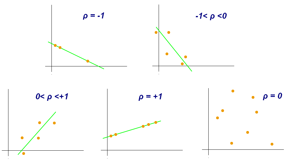
If you had tried calculating the Pearson correlation coefficient (PCC) in DAX, you would have likely read Gerhard Brueckl’s excellent blog post. If you haven’t, I encourage you to read it, as it contains a high-level overview of what PCC is. In this article I am showing how the same calculation can be done more efficiently using the new DAX functions, which are available starting with Power Pivot in Excel 2016, Power BI Desktop, SQL Server 2016 Analysis Services, and Azure Analysis Services.
The new DAX functions allow us to compute PCC in just one easy-to-use measure. Furthermore, depending on your data model, you may see a significant performance improvement. I have tested the new approach on two data models, and in one of them the calculation ran 93% faster, while the other model saw only a 20% increase in performance. The comparison is not exactly fair though, because the new formula has one additional benefit: it treats missing values in the same way as Excel’s CORREL function.
To illustrate the last point, let’s have a look at the very basic data model below:
| Item | Value X | Value Y |
| A | 2 | 0 |
| B | 3 | 1 |
| C | 5 | 1 |
| D | 7 | 2 |
If we calculate the correlation coefficient between Value X and Value Y using the CORREL function in Excel, we will get 0.92, and we will get the same result by following Gerhard’s approach in DAX. So far, so good.
However, if we remove one of the values, the calculations will no longer match. For example, let’s remove the number seven from our data.
| Item | Value X | Value Y |
| A | 2 | 0 |
| B | 3 | 1 |
| C | 5 | 1 |
| D | 2 |
Now the CORREL function returns 0.76 and the original formula returns -0.39. Note that Excel treats missing values differently from zeros. Essentially, Excel ignores the whole pairs where at least one value is missing. If we replaced 7 with 0, we would get -0.39 — same as using Gerhard’s formula.
The new DAX correlation coefficient formula matches Excel’s logic. Here is the DAX formula:
Correlation Coefficient :=
VAR Correlation_Table =
    FILTER (
        ADDCOLUMNS (
            VALUES ( 'Table'[Column] ),
            "Value_X", [Measure_X],
            "Value_Y", [Measure_Y]
        ),
        AND (
            NOT ( ISBLANK ( [Value_X] ) ),
            NOT ( ISBLANK ( [Value_Y] ) )
        )
    )
VAR Count_Items =
    COUNTROWS ( Correlation_Table )
VAR Sum_X =
    SUMX ( Correlation_Table, [Value_X] )
VAR Sum_X2 =
    SUMX ( Correlation_Table, [Value_X] ^ 2 )
VAR Sum_Y =
    SUMX ( Correlation_Table, [Value_Y] )
VAR Sum_Y2 =
    SUMX ( Correlation_Table, [Value_Y] ^ 2 )
VAR Sum_XY =
    SUMX ( Correlation_Table, [Value_X] * [Value_Y] )
VAR Pearson_Numerator =
    Count_Items * Sum_XY - Sum_X * Sum_Y
VAR Pearson_Denominator_X =
    Count_Items * Sum_X2 - Sum_X ^ 2
VAR Pearson_Denominator_Y =
    Count_Items * Sum_Y2 - Sum_Y ^ 2
VAR Pearson_Denominator =
    SQRT ( Pearson_Denominator_X * Pearson_Denominator_Y )
RETURN
    DIVIDE ( Pearson_Numerator, Pearson_Denominator )
To use the formula, simply replace:
- The red part with a table expression that returns the items for which you calculate your measures X and Y
- The green part with your measure X
- The blue part with your measure Y
You can also insert the formulas for [Measure_X] and [Measure_Y] directly into the code above — just don’t forget to wrap them in CALCULATE to trigger context transition.
If you think this pattern is useful, please give kudos to it in the Quick Measures Gallery.
Sample Excel 2016 workbook: Correlation.xlsx