Linear regression in DAX

Random data points and a simple linear regression line

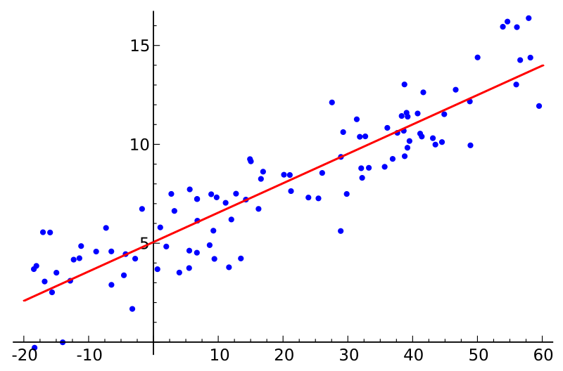
DAX, originating in Power Pivot, shares many functions with Excel. As of 2017, some of the functions, such as SLOPE and INTERCEPT, exist in the latter but not in the former. The two functions can be used for a simple linear regression analysis, and in this article I am sharing patterns to easily replicate them in DAX. But first, why would you want to do such analysis?

Update 28 February 2023: LINESTX is now used to calculate the slope and intercept. Note that LINEST and LINESTX allow you to perform multiple linear regression as well!

Update 2 December 2017: the sales example was updated to display the correct Estimated Sales figure at the grand total level.

How can I use simple linear regression?

With simple linear regression, you can estimate the quantitative relationship between any two variables. Let’s say you have the following data model:

Name Height (cm) Weight (kg)
Harry 166 54
Hermione 164 51
Ron 173 73
Ginny 171 55
Dumbledore 181

Note how Dumbledore’s weight is unknown — we are going to predict it with simple linear regression.

Linear regression has been done in DAX before (by Rob Collie and Greg Deckler, for instance), but my approach uses the new DAX syntax, which makes the calculations very easy.

Simple linear regression pattern

Simple linear regression can be done in just one measure:

Simple linear regression =
VAR Known =
    FILTER (
        SELECTCOLUMNS (
            ALLSELECTED ( Table[Column] ),
            "Known[X]", [Measure X],
            "Known[Y]", [Measure Y]
        ),
        AND (
            NOT ( ISBLANK ( Known[X] ) ),
            NOT ( ISBLANK ( Known[Y] ) )
        )
    )
VAR SlopeIntercept =
    LINESTX(Known, Known[Y], Known[X])
VAR Slope =
    SELECTCOLUMNS(SlopeIntercept, [Slope1])
VAR Intercept = 
    SELECTCOLUMNS(SlopeIntercept, [Intercept])
RETURN
    Intercept + Slope * [Measure X]

To make it work for you, replace the

  1. Red part with your category values column reference
  2. Green parts with your independent values measure (twice)
  3. Blue part with your dependent values measure

Estimating Dumbledore’s weight

We can now estimate Dumbledore’s weight and, with a little more DAX, build the following graph:

Dumbledore's weight is highlighted as estimated one

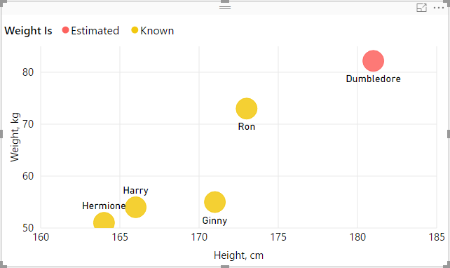
Note how we show known weight values when weight is known, but we display estimated weight in case where weight is not known.

Other ways to use the pattern

You are not limited to using measures for known X and Y values — you can also use columns, thanks to row context being present in SELECTCOLUMNS. For example, to estimate future sales, you can use dates in place of Measure X, like so:

Simple linear regression =
VAR Known =
    FILTER (
        SELECTCOLUMNS (
            ALLSELECTED ( 'Date'[Date] ),
            "Known[X]", 'Date'[Date],
            "Known[Y]", [Measure Y]
        ),
        AND (
            NOT ( ISBLANK ( Known[X] ) ),
            NOT ( ISBLANK ( Known[Y] ) )
        )
    )
VAR SlopeIntercept =
    LINESTX(Known, Known[Y], Known[X])
VAR Slope =
    SELECTCOLUMNS(SlopeIntercept, [Slope1])
VAR Intercept = 
    SELECTCOLUMNS(SlopeIntercept, [Intercept])
RETURN
    SUMX (
        DISTINCT ( 'Date'[Date] ),
        Intercept + Slope * 'Date'[Date]
    )

Note that to display the correct amount at the grand total level, you also need to modify the RETURN expression. In case of sales, it is appropriate to use SUMX; if you deal with temperatures, for example, you will probably use AVERAGEX.

You can then build the following graph:

Actual and estimated sales on one graph

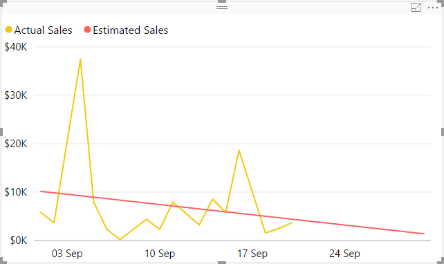
The red line looks a lot like a trend line, doesn’t it? In fact, if you add a trend line to the graph, it will be exactly the same as red line:

Actual and estimated sales with trend line

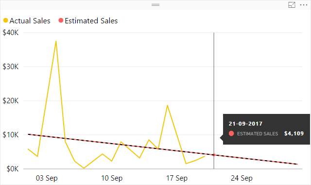
There are at least two reasons to consider calculated trend lines:

  1. With the built-in trend line, you can only infer its values from the Y axis, while the calculated trend line allows you to see the values explicitly
  2. As of September 2017, Power BI allows you to only add trend lines for numeric or datetime axes. As soon as you use strings (month names, for instance), you lose the ability to add trend lines. With simple linear regression, you can calculate them yourself, as long as you have sequential numeric values to use as known X values

If you think this pattern is useful, please give kudos to it in the Quick Measures Gallery.

Happy forecasting!

Sample Power BI file: Simple linear regression.pbix

  • Mim

    wow, this is brilliant !!!!

  • Mack Cage

    Good Stuff thanks!

  • Rainar Essenson

    Hi Daniil!

    Great job with combining all the variables in one measure!
    I have a question though – what if i want to show Sales Estimate on a different value then Date.
    Instead of ‘date’ values I added ‘Date'[Month Name] but got an error, that SUMX cannot work with ‘string’ values. I did try using numeric values from ‘Date’ table (like month number & relative month) – these work well, but on the visual I’d like to show [Month Name] – unfortunately it does not calculate correctly if i use y-axis as something different then the column selection I have made in the measure.

    Anyway my goal is to show sales per customer for the past selected period (usually rolling 12 months) and then give an indication if sales trend is going up or down based on the ‘slope’ variable. But I also want to show the actual trend line on the visual using a user friendly format (January 2018).

    • Hi, Rainar, thanks for your question! You can try the following formula (note the changes in the Known variable and the RETURN statement):
      Estimated Sales =
      VAR Known =
      FILTER (
      SELECTCOLUMNS (
      SUMMARIZE (
      ALLSELECTED ( 'Date' ),
      'Date'[Calendar Year Month],
      'Date'[Calendar Year Month Sequential Number]
      ),
      "Known[X]", 'Date'[Calendar Year Month Sequential Number],
      "Known[Y]", [Sales Amount]
      ),
      AND (
      NOT ( ISBLANK ( Known[X] ) ),
      NOT ( ISBLANK ( Known[Y] ) )
      )
      )
      VAR Count_Items =
      COUNTROWS ( Known )
      VAR Sum_X =
      SUMX ( Known, Known[X] )
      VAR Sum_X2 =
      SUMX ( Known, Known[X] ^ 2 )
      VAR Sum_Y =
      SUMX ( Known, Known[Y] )
      VAR Sum_XY =
      SUMX ( Known, Known[X] * Known[Y] )
      VAR Average_X =
      AVERAGEX ( Known, Known[X] )
      VAR Average_Y =
      AVERAGEX ( Known, Known[Y] )
      VAR Slope =
      DIVIDE (
      Count_Items * Sum_XY - Sum_X * Sum_Y,
      Count_Items * Sum_X2 - Sum_X ^ 2
      )
      VAR Intercept =
      Average_Y - Slope * Average_X
      RETURN
      SUMX (
      DISTINCT ( 'Date'[Calendar Year Month Sequential Number] ),
      Intercept + Slope * 'Date'[Calendar Year Month Sequential Number]
      )

      You just need to make sure that the sorting column consists of sequential numbers. By that I mean it is “year * 12 + month”, not “year * 100 + month”.

      • Rainar Essenson

        Thank you Daniil! Спасибо 😉
        I did try using ‘relative month’ (Current month = 0, previous month = -1 etc) field from my date table, but that did not work out that well – so yes I created month sequence in my date table.
        I ended up multiplying my sales slopes with sales amount in order to also take account the magnitude of change in trend. From that number I created dynamic segments – aggressive/moderate/flat/declining etc. The outcome is quite interesting – possible to filter customers according to their past sales trend.
        Not completely sure how my data holds up to being evaluated on a linear trend – daily sales are fluctuating a lot, monthly looks better in this case.

        Thanks again for your help! I really like your blog posts!

        • Your multiplication of slope and sales amount with subsequent dynamic segmentation sounds like a very interesting application of linear regression. You should consider writing a blog post about it 🙂

          Aitäh for your feedback, Rainar!

      • knyazs

        Hi Daniil,
        Thanks again for very useful example. I tried the code above (on a Year granularity) using sequential Epoch values for years (2010 = 1262304000, 2011 = 1293840000, 2012 = 1325376000 and so on) and I modified the code as per your suggestion, but I am getting value for the trend to be equal to value of a measure (Y).
        Then, I created only a measure to show Count_Items and I got following result:

        Year | Count_Items
        2017 | 1
        2018 | 1
        2019 | 1

        Should not it be:
        Year | Count_Items
        2017 | 3
        2018 | 3
        2019 | 3

        My code looks like this:

        Utilization Trend 3 [Final]:=
        VAR Known =
        FILTER (
        SELECTCOLUMNS (
        SUMMARIZE(
        ALLSELECTED('Date'),
        'Date'[Year],
        'Date'[YearEpoch]
        ),
        "Known[X]", 'Date'[YearEpoch],
        "Known[Y]", [Utilization]
        ),
        AND ( NOT ( ISBLANK ( Known[X] ) ), NOT ( ISBLANK ( Known[Y] ) ) )
        )

        VAR Count_Items =
        COUNTROWS ( Known )
        VAR Sum_X =
        SUMX ( Known, Known[X] )
        VAR Sum_X2 =
        SUMX ( Known, Known[X] ^ 2 )
        VAR Sum_Y =
        SUMX ( Known, Known[Y] )
        VAR Sum_XY =
        SUMX ( Known, Known[X] * Known[Y] )
        VAR Average_X =
        AVERAGEX ( Known, Known[X] )
        VAR Average_Y =
        AVERAGEX ( Known, Known[Y] )
        VAR Slope =
        DIVIDE (
        Count_Items * Sum_XY - Sum_X * Sum_Y,
        Count_Items * Sum_X2 - Sum_X ^ 2
        )
        VAR Intercept =
        Average_Y - Slope * Average_X
        RETURN
        SUMX (
        DISTINCT ( 'Date'[YearEpoch] ),
        Intercept + Slope * 'Date'[YearEpoch]
        )

        • Can you please share a sample .pbix file? Without it, my only guess is that you are either sorting [Year] by something other than [YearEpoch], or there are some other filters at play.

          • knyazs

            Thank you for the quick reply. Before I share the report (I am using SSAS cube behind the scenes so it will take me some time to prepare it), can you just help me understanding how this should work?

            For example, let’s say we have 5 measures in 2 years:
            Date | Measure
            – Jan 2017 | 4
            – Jul 2017 | 3
            – Jan 2018 | 6
            – Jul 2018 | 8
            – Jan 2019 | 7

            Let’s just focus on Count_Items for now. If I use the example you gave for Known table:

            Code #1
            SELECTCOLUMNS (
            ALLSELECTED ( ‘Date'[Date] ),
            “Known[X]”, ‘Date'[Date],
            “Known[Y]”, [Measure Y]
            ),

            I would get the following:

            ‘Date'[Date] | Count_Items
            Jan 2017 | 1
            Jul 2017 | 1
            Jan 2018 | 1
            Jul 2018 | 1
            Jan 2019 | 1

            Which I assume is wrong. But, if I use following syntax for Known:

            Code #2
            SELECTCOLUMNS (
            ALLSELECTED ( ‘Date’ ),
            “Known[X]”, ‘Date'[Date],
            “Known[Y]”, [Measure Y]
            ),

            I would get, presumably, correct result:
            ‘Date'[Date] | Count_Items
            Jan 2017 | 5
            Jul 2017 | 5
            Jan 2018 | 5
            Jul 2018 | 5
            Jan 2019 | 5

            This works fine for date level of granularity, but when I want to aggregate on Year level, SUMMARIZE essentially does the calculation the same way as example 1 I showed and I am getting the following:

            Code #3
            SELECTCOLUMNS (
            SUMMARIZE (
            ALLSELECTED ( ‘Date’ ),
            ‘Date'[Year],
            ‘Date'[YearSeq]
            ),
            “Known[X]”, ‘Date'[YearSeq],
            “Known[Y]”, [Measure]
            ),

            ‘Date'[Year] | Count_Items
            2017 | 1
            2018 | 1
            2019 | 1

            where it should be:
            ‘Date'[Year] | Count_Items
            2017 | 3
            2018 | 3
            2019 | 3

            Can SUMMARIZE somehow be written in the same way I wrote Code #2?

            Btw, can you please share your email so that I can send you sample PowerBI report?

            Thanks,

          • knyazs

            I found a solution for this – because of the way the cube is designed, I had to wrap Known variable with:

            VAR Known_Y = CALCULATETABLE(
            FILTER (
            SELECTCOLUMNS (
            SUMMARIZE(
            ALLSELECTED('Date'),
            'Date'[YearSeq]
            ),
            "Known_Y[X]", 'Date'[YearSeq],
            "Known_Y[Y]", [Measure]
            ),
            AND (
            NOT(ISBLANK(Known_Y[X])),
            NOT(ISBLANK(Known_Y[Y]))
            )
            )
            , ALLSELECTED('Date')
            )

            After adding this, everything worked fine.

          • Ana Cristina Aranda

            Hi knyazs,

            I had the same problem and I solved it using your solution. Did you understand why sometimes it Works without wrap Known variable and sometimes it does not work?

            Thanks for share with us your solution.

  • Prashanth Mohan

    Hi Daniil,

    Thanks for the post. It is really very helpful. But, I wanted to know if it is possible to have this regression line for separate time frames.

    Say, a regression line from 3rd sep to 10th sep. another regression line from 10th sep to 17th Sep..

    I wanted to show trends for each time-frame in my chart in power BI, wanted to know if that is achievable?

    Thanks and Regards,
    Vishnu

    • Hello, Prashanth. Yes, I think what you want is possible, though it’s not going to look great, in my opinion, because different segments will still be connected: https://uploads.disquscdn.com/images/19e1e2540ab640b1c3b720464d224e6fd49be01e006c7154bfd9eed2a04ceed9.png

      Here is one way you could do this:
      Estimated Sales 2 =
      VAR ThisWeek =
      WEEKNUM ( SELECTEDVALUE ( ‘Date'[Date] ), 2 )
      VAR Known =
      FILTER (
      SELECTCOLUMNS (
      FILTER ( ALLSELECTED ( ‘Date'[Date] ), WEEKNUM ( ‘Date'[Date], 2 ) = ThisWeek ),
      “Known[X]”, ‘Date'[Date],
      “Known[Y]”, [Actual Sales]
      ),
      AND ( NOT ( ISBLANK ( Known[X] ) ), NOT ( ISBLANK ( Known[Y] ) ) )
      )
      VAR Count_Items =
      COUNTROWS ( Known )
      VAR Sum_X =
      SUMX ( Known, Known[X] )
      VAR Sum_X2 =
      SUMX ( Known, Known[X] ^ 2 )
      VAR Sum_Y =
      SUMX ( Known, Known[Y] )
      VAR Sum_XY =
      SUMX ( Known, Known[X] * Known[Y] )
      VAR Average_X =
      AVERAGEX ( Known, Known[X] )
      VAR Average_Y =
      AVERAGEX ( Known, Known[Y] )
      VAR Slope =
      DIVIDE (
      Count_Items * Sum_XY
      – Sum_X * Sum_Y,
      Count_Items * Sum_X2
      – Sum_X ^ 2
      )
      VAR Intercept = Average_Y
      – Slope * Average_X
      RETURN
      Intercept
      + Slope * SELECTEDVALUE ( ‘Date'[Date] )

  • Jaime Cueva

    Very good…

  • Jan

    Thank you Daniil,

    Very elegant and powerful. It would be useful to add the standard error of the regression / standard error of the estimate (Excel function STEYX). Basically a the standard deviation around the Estimated sales trend line?

    • I would need to think about how this would be done — I think that would be a good addition 🙂

  • Bojan Makivic

    This is aaaaawesome 🙂 Great work Daniil!!!

    Is it possible to adapt this DAX code for multiple regression analysis (with more independent variables)???
    Tanks.

  • knyazs

    Awesome! I used this code to create a sample report on simple SUM measure from Excel, and it worked flawlessly. Now, I am trying to do the same on the proper dimensional model with Dim Date and Fact tables and I am unable to make it work – if I add a Date field into the fact table, then it works, but if I use Date field from DimDate, calculation does not work. What am I missing here? Just to mention that DimDate and Fact have proper relation created between Date Surrogate Keys on both tables.

    • Would you be willing to share a sample dataset? Otherwise it’s a bit difficult to suggest anything meaningful.

      • knyazs

        Hi Daniil, thank you for quick response. Sample datasets are Fact table and standard DimDate table connected to the Fact table by 1 to many relationship through integer surrogate key. Literary moments ago I managed to find a solution by replacing ‘ALLSELECTED ( ‘Date'[Date] )’ with ‘ALLSELECTED ( ‘Date’ ),’.

  • Mike Richards

    This is great! I had a few questions.
    This works strictly on the date level, but I really need it on Month / Quarter level. I tried to follow the other post with the month sort column but I cant seem to get it to come out at all.
    also, when I crossfilter for a customer on the report pane in a separate table, the trend no longer matches up. How can I account for that to make sure the regressions line up with each account as well? Thanks in advance!!!

    • It’s a bit difficult to diagnose based on your comment — would you mind sharing a sample file? The only piece of advice I can offer right now is that you should use a sorting column that uniquely identifies a month in any year — i.e., YearMonth sorting column.

      • Mike Richards

        Thanks for the quick reply! I figured out the first one with the crossfiltering. the question I have left is that the Regression only works with the month sort field, instead of a the date or the month field to get a visualization with a recognizable date field.
        link to sample pbix of how my data is set up. one visual is what it looks like with a date field, and one with the months sort field that works correctly.

  • Raymond Pocher

    Hey There, first of all, great work! This is really something and very sophisticated. I have 2 questions: How can that be achieved on a monthly basis? Now that you have the trend, would it be possible to combine the trend line with seasonal information of the data to get an even more accurate regression?

    • Adding seasonality is possible — it would just require more lines of code. Also, you would need to decide between additive and multiplicative decomposition. The following link might be useful to you: https://otexts.com/fpp2/components.html

      • Raymond Pocher

        Hehe, Thank you! I am not sure if I can get through this. Perhaps, in a moment of boredom, you dedicate a little time to this. I guess many people would appreciate this. I sort of know how to do it in excel but not in dax :/

  • Alex Bergman

    Daniil,

    Could you tell me how to find a specific future value from the measure? For example, I used your DAX to create a regression line for sales$ over time. I want to create a measure to calculate the sales on the last day of next month using the regression measure I created from your DAX. I need it to be a measure so that I can use it in other subsequent measures.

    My current DAX formula is as follows:

    FUTURE_MONTH_1_SALES = CALCULATE(‘SALES_FACT'[SIMPLE_LINEAR_REGRESSION],’CALENDAR_DIM'[DATE_DESC] = (EOMONTH(TODAY(),1)))

  • Matthew Smith

    This is really awesome Daniil. However, I am getting the below error.

    MdxScript(Model) (208,37) Calculation error in measure ‘DimDate'[_PreviousDate12mo]: An argument of function ‘DATE’ has the wrong data type or the result is too large or too small.

    Did you experience any similar errors? My measure is a rolling 12-month rate

  • mmmgaus

    Hi Daniil, great work! I’m new to Power Bi and DAX. Could you please show the code needed to replicate Power BI’s combine series ‘Off’. I have two series – one for each product as shown in the screenshot below:
    https://uploads.disquscdn.com/images/7df9e1d03e990f5e8f071c672111faeac795e4ccd65b7bafe378da1528046309.png https://uploads.disquscdn.com/images/7df9e1d03e990f5e8f071c672111faeac795e4ccd65b7bafe378da1528046309.png
    This is my code –
    Measure 2 =
    VAR Known =
    Filter(
    SELECTCOLUMNS(
    ALLSELECTED (Sheet1[MonthYear],Sheet1[Product Category]),
    “Known[X]”, Sheet1[MonthYear],
    “Known[Y]”, [Measure]
    ),
    AND (NOT(ISBLANK(Known[X])), NOT(ISBLANK(Known[Y]))))
    VAR Count_Items = COUNTROWS(Known)
    VAR Sum_X = SUMX(Known, Known[X])
    VAR Sum_X2 = SUMX(Known, Known[X]^2)
    VAR SUM_Y = SUMX(Known, Known[Y])
    VAR SUM_XY = SUMX(Known, Known[X] * Known[Y])
    VAR Average_X = AVERAGEX(Known, Known[X])
    VAR Average_Y = AVERAGEX(Known, Known[Y])
    VAR Slope = DIVIDE(Count_Items * SUM_XY – Sum_X * SUM_Y, Count_Items * Sum_X2 – Sum_X^2)
    VAR Intercept = Average_Y – Slope * Average_X
    Return SUMX(DISTINCT(Sheet1[MonthYear]), Intercept + Slope * Sheet1[MonthYear])

    but I think it’s combining both series into 1 trend line – I need a separate trend line for each product:

    Thank you.

    • mmmgaus

      Hi Daniil,
      it’s ok. I just created two separate measures as follows:
      Measure 2 =
      VAR Known =
      Filter(
      SELECTCOLUMNS(
      ALLSELECTED (Sheet1[MonthYear],Sheet1[Product Category]),
      “Known[X]”, Sheet1[MonthYear],
      “Known[Y]”, [Measure],
      “Known[Z]”, Sheet1[Product Category]
      ),
      AND(AND(NOT(ISBLANK(Known[X])), NOT(ISBLANK(Known[Y]))), Known[Z] = “Financial Lines”))
      VAR Count_Items = COUNTROWS(Known)
      VAR Sum_X = SUMX(Known, Known[X])
      VAR Sum_X2 = SUMX(Known, Known[X]^2)
      VAR SUM_Y = SUMX(Known, Known[Y])
      VAR SUM_XY = SUMX(Known, Known[X] * Known[Y])
      VAR Average_X = AVERAGEX(Known, Known[X])
      VAR Average_Y = AVERAGEX(Known, Known[Y])
      VAR Slope = DIVIDE(Count_Items * SUM_XY – Sum_X * SUM_Y, Count_Items * Sum_X2 – Sum_X^2)
      VAR Intercept = Average_Y – Slope * Average_X
      Return SUMX(DISTINCT(Sheet1[MonthYear]), Intercept + Slope * Sheet1[MonthYear])

      Measure 3 =
      VAR Known =
      Filter(
      SELECTCOLUMNS(
      ALLSELECTED (Sheet1[MonthYear],Sheet1[Product Category]),
      “Known[X]”, Sheet1[MonthYear],
      “Known[Y]”, [Measure],
      “Known[Z]”, Sheet1[Product Category]
      ),
      AND(AND(NOT(ISBLANK(Known[X])), NOT(ISBLANK(Known[Y]))), Known[Z] = “Accident & Health”))
      VAR Count_Items = COUNTROWS(Known)
      VAR Sum_X = SUMX(Known, Known[X])
      VAR Sum_X2 = SUMX(Known, Known[X]^2)
      VAR SUM_Y = SUMX(Known, Known[Y])
      VAR SUM_XY = SUMX(Known, Known[X] * Known[Y])
      VAR Average_X = AVERAGEX(Known, Known[X])
      VAR Average_Y = AVERAGEX(Known, Known[Y])
      VAR Slope = DIVIDE(Count_Items * SUM_XY – Sum_X * SUM_Y, Count_Items * Sum_X2 – Sum_X^2)
      VAR Intercept = Average_Y – Slope * Average_X
      Return SUMX(DISTINCT(Sheet1[MonthYear]), Intercept + Slope * Sheet1[MonthYear])

      The result is:

      https://uploads.disquscdn.com/images/14185445567fe64f7dc29f0420b636bd6c6e05759e1427712313da69c7749627.png

  • Marcos Pérez del Hierro

    Hi all, This is not working for me, the output are the values of my measure instead of a trend line: https://uploads.disquscdn.com/images/765ca66611ac0e889230a7e002e655a56bf55e30cb4031c4b537471f6476967f.png

    This is my code:

    Simple linear regression =
    VAR Known =
    FILTER (
    SELECTCOLUMNS (
    ALLSELECTED ( Merge1[Fecha] );
    “Known[X]”; Merge1[Fecha];
    “Known[Y]”; SUM(Merge1[Posevento])
    );
    AND (
    NOT ( ISBLANK ( Known[X] ) );
    NOT ( ISBLANK ( Known[Y] ) )
    )
    )
    VAR Count_Items =
    COUNTROWS ( Known )
    VAR Sum_X =
    SUMX ( Known; Known[X] )
    VAR Sum_X2 =
    SUMX ( Known; Known[X] ^ 2 )
    VAR Sum_Y =
    SUMX ( Known; Known[Y] )
    VAR Sum_XY =
    SUMX ( Known; Known[X] * Known[Y] )
    VAR Average_X =
    AVERAGEX ( Known; Known[X] )
    VAR Average_Y =
    AVERAGEX ( Known; Known[Y] )
    VAR Slope =
    DIVIDE (
    Count_Items * Sum_XY – Sum_X * Sum_Y;
    Count_Items * Sum_X2 – Sum_X ^ 2
    )
    VAR Intercept =
    Average_Y – Slope * Average_X
    RETURN
    SUMX(
    DISTINCT(Merge1[Fecha]);
    Intercept+Slope*Merge1[Fecha])

    Thanks!

    • Ana Cristina Aranda

      Hi Marcos, did you solve this? When I used this aproach for the first time it was happening to me, too. I solved this creating a measure for my known Y value instead of using the whole expression… for your code it should be something like:

      Measure Total Posevento = SUM(Merge1[Posevento])

      And use this measure in the SELECTCOLUMNS function ….

      It worked for me

      • Aishwar

        Hi Ana
        Even I am facing the same problem, the DAX generates the values as the original measure. I have a single table with a date and all the values and in X-axis I have a custom column like Fy20219.

  • aman

    Hi Daniil can you please help me with DAX for the trendline. I have a customised date column and for your refrence i have attached the screenshot of my graph. https://uploads.disquscdn.com/images/1a5b3897c7df6b96ad53e8a2d36ffb046b922185192970e99d196fb38cd50e66.png

  • sherifffruitfly

    Very nice!

    I’m trying to fit an exponential curve via the log transform – so I’m feeding in Known[Y] as ln(ActualValues).

    Am I following your code correctly in concluding that undoing the log transform in the return looks like:


    RETURN
    SUMX (
    DISTINCT ( 'Calendar'[Date] ),
    exp(Intercept + Slope * 'Calendar'[Date])
    )

    ?

  • Денис Раневский

    Thank you. Great work! But how i can see angle of trendline? It possible?

  • christine

    Hi, my linear regression line do not become linear

  • Satish

    Could you please tell me how to calculate logarithmic regression ?